
Firstly i would like to apologize for the lack of content the past month, I have been working on a lot of academic related material, and been constructing this system. This rating system is the most mathematically complex one I have constructed to this date, therefore I welcome any questions regarding it. It actually involved two metrics, one is a new way to look at margin of victory, and the other takes a lot from Ken Massey’s esteemed rating system. I will also be using this system for College Football teams currently, however it can be used for practically any sport!
Part 1: Time Adjusted Margin(TAM)
The most contemporary way to look at how dominant a team is in any sport, is the Margin of Victory. Which is simply subtracting the opponent’s points from the team’s points. It is a controversial metric in the realm of advanced ratings, as it can overvalued teams that run up the score. However, I am of the opinion, that it is a necessary aspect. If Team B and C both beat Team A, but team B wins by 28 while Team C wins by 3, those wins should not be counted the same.
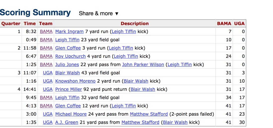
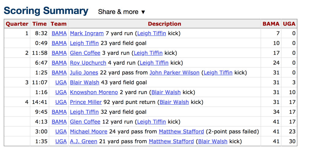
Another flaw of basic margin of victory is that it can be misleading. Teams that go up by 3 or 4 scores early, will often sub in their second and third strings which allows other teams to score garbage time touchdowns. A prime example of this would be 2008 Alabama’s showdown vs. #3 Georgia. The Final score was 41-30, which gives the impression Alabama pulled away at the end, however that was simply not the case. The Crimson Tide went up 31-0 in the first half and were up 41-17 with four minutes left in the fourth.
On the other end a highly contested matchup, with the opposing teams going back and forth, can seem lopsided when just looking at the final score. A prime example, also coming from Alabama, was their 37-21 win over Texas in the 2009 season’s national title game. Star quarterback Colt McCoy went down for the Longhorns early, and despite this, the score was 24-21 prior to the 2: 00-minute mark in the last quarter. Fluke instances or team’s trying to put the game away can make a back and forth contest seem lopsided.
This is why I created Time Adjusted Margin, which is calculated based on the following:
(60-(Final time in the game when team went up by more than 8 Points)
The essence is not entirely clear just based on the formula, therefore I will use some examples.
The raw, time-adjusted margin would be 46, because Alabama went up 10-0 at the 1 minute mark in the first, with 46 minutes left in the game. An important thing to remember is that, if Georgia had gotten the score to 31-24 at some point in the game, it would have been different. The metric is based on the time the team went up by more than one possession, and never relinquished that 1+ possession lead for the entirety of the game. While Georgia would have had a margin of -46.
The raw, time-adjusted margin in this game would have been 2 because Alabama went up by 10 at the 2:01 mark in the fourth, not 30 despite the fact they went up by 11 at the 29 second mark in the second quarter.
Some Adjustments that should be noted:
-Games that finish within one score are assigned a rating of 5, to still provide emphasis on winning, even if it came in the last minutes. Also teams who go up by more than one possession within the 5 minute mark in the fourth, are also assigned a 5.
there is a home/away adjustment which is +/- 3.43, this is based on the least squares regression equation of, and the 2.5 standard home-field advantage usually used by odds makers:
y=1.31x+0.15
x being the Time margin with y being the margin of victory.
Part 2: TIMEMAT
This system is based on Kenneth Massey’s Matrix system in which he uses the linear algebra least squares equation of:

To fully understand the mathematics behind this, one should most likely have some sort of experience in Linear Algebra. However I will try my best to explain it in such way, where one will get a decent idea of it no matter their background. The whole point of this site, is to remove the ambiguity involving advanced metrics, and give readers insight into what they are actually seeing when they see metrics thrown around. If you are intrigued by this I would highly recommend the book: The Science of Rating and Ranking Who’s #1 by Amy N. Langville and Carl D. Meyer. They do a great job at explaining the system that Massey uses!
When looking at larger sample sizes, it is nearly impossible to look at matrices just as a system of linear equations, therefore I will use the games played between Texas, Texas Tech, Oklahoma and Oklahoma State in the 2008 Big 12 South.
The Games resulted in the following:
Texas beating Oklahoma in a neutral site TAM: 5.0
Oklahoma beating Texas Tech at Home TAM: 40.57
Oklahoma beating OK State on the Road TAM: 10.43
Texas beating OK State at home TAM: 1.57
Texas Tech beating Texas at home TAM: 1.57
Texas Tech beating OK State at home TAM: 27.57
You start off with a Matrix m (games played) x n (# of teams) matrix, X. You are trying to solve for the system Xr=y where x is a team, r are the ratings you are trying to calculate, and y is the list of Time Adjusted Margins of each game. (X1=Oklahoma, X2=Texas, X3=Texas Tech, X4=OK State)
OU vs. Texas: -1×1+1×2+0x3+0x4=5
OU vs. Texas Tech: 1×1+0x2-1×3+0x4=40.57
OU vs. OK State: 1×1+0x2+0x3-1×4=1.57
Texas vs. OK State: 0x1+1×2+0x3-1×4=1.57
Texas Tech vs. Texas: 0x1-1×2+1×3+0x4=1.57
Texas Tech vs. OK State: 0x1+0x2+1×3-1×4=27.57
If you could not tell already, a team that wins the game gets a 1 and the team that loses gets a -1, and a team not involved in that particular match-up has a coefficent of 0.
You then transpose this where the rows become the columns, and vice versa, which looks like
OU:-1w1+1W2+1w3+0w4+0w5+0w6
Texas: 1w1+0w2+0w3+1w4+-1w5+0w6
Texas Tech: 1w1+0w2+0w3+1w4-1w5+0w6
OK State: 0w1+0w2-1w3-1w4+0w5-1w6
the w’s here are each game played, which is why some teams have a coefficient for each w while others don’t because obviously Texas Tech was not involved in the Texas Oklahoma Game. Then I use matrix multiplication to multiply this system by the previous system and set it equal to XT times the Y Vector which simply becomes the cumulative Time Margins of each team, which turns into :
3×1-1×2-1×3-1×4=46
-1×1+3×2-1×3-1×4=5
-1×1-1×2+3×3-1×4=-11.43
-1×1-1×2-1×3-1×4=-39.57
It is hard to see how this equation has any merit without understanding linear algebra. In summation, it simply creates n x n square matrix, that builds dependence within it. In the sense that the matrix inherently accounts for such things, as the strength of schedule. The process is trying to simply find the closest set of ratings that accounts for the given data of a team beating certain team given a certain time margin.
Massey uses an adjustment to make the matrix invertible, and something that in a way scales it by making one of the lines all 1s, and the corresponding entry in the Y vector, to Zero. The mathematics behind this are based in the fact, that no matter how the schedule works out (even if they play a team multiple times), the sum of the rows is 0. This means that the all ones vector is in the null space of the matrix, and maps the system to the zero vector. If one replaces an arbitrary row of the coefficents with all ones, and a zero on the right. This set of ones, is no longer in the solution set as the right side gives M (# of teams and not zero). The Matrix’s other entries are based on the other team’s results therefore one can replace any row and still yield the same results:
Solving the system using Gaus-Jordan Elimination:
(3×1-1×2-1×3-1×4)*R1=46
(-1×1+3×2-1×3-1×4)*R2=5
(-1×1-1×2+3×3-1×4)*R3=-11.43
(1×1+1×2+1×3+1×4)*R4=0
yields these ratings:
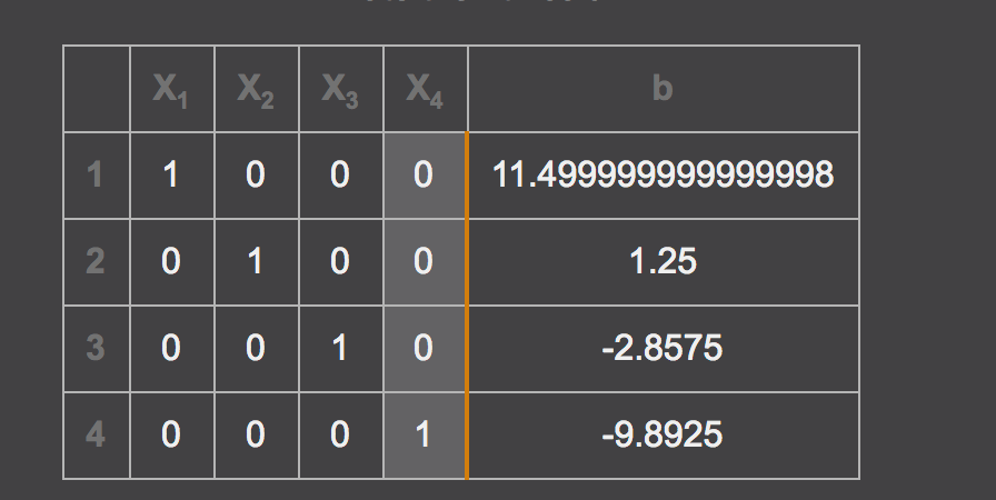
1. Oklahoma 11.50
2. Texas 1.25
3. Texas Tech -2.86
4. OK State: -9.89
Keep in mind, this small sample size is based simply on the games played between the two teams, and the ratings would be different if you expanded it to the entirety of the season.
These ratings can be used to predict the outcome of games, if Oklahoma had played Texas Again, the metric would predict Oklahoma to go up by more than 1 poss. at 10 minute mark in the fourth quarter since (11.50-1.25-10.25), which translates to a pretty close game.
I also calculated the ratings for the SEC teams based solely on their conference games this year:
which gave the results:
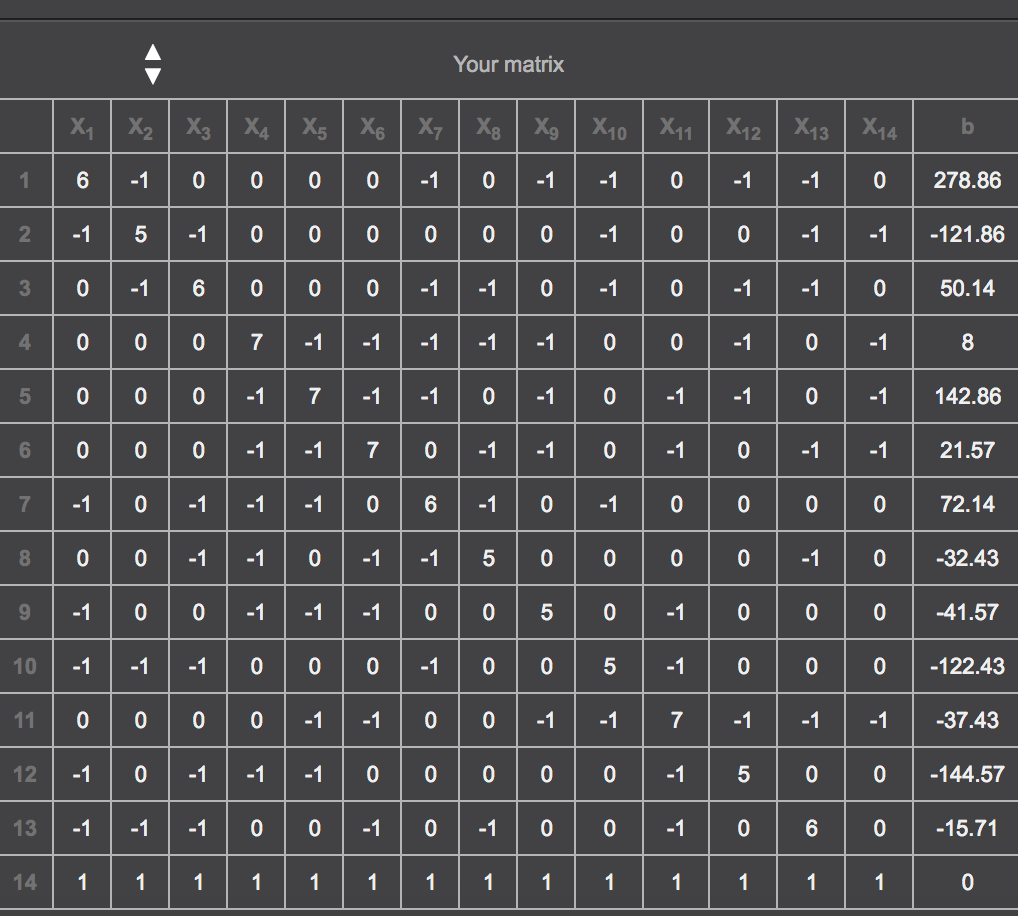
The order of the teams were as followed in the matrix: Alabama, Ark, Auburn, Florida, Georgia, Kentucky, LSU, Miss State, Ole Miss, Mizzou, SC, Tennessee, TAMU, Vandy.
1. Alabama 39.8
2. LSU 18.83
3. Georgia 18.33
4. Kentucky 2.79
5. Mizzou 2.48
6. Florida 2.43
7. Auburn 0.99
8. TAMU -1.10
9. Miss State -1.68
10. South Carolina -13.25
11. Vanderbilt -13.25
12. Vols -18.48
13. Ole Miss -19.01
14. Arkansas -22.87
In summation: This rating system solves the equation in the closest way possible: of ra-rb=t, where RA is the rating of Team A, and RB is the rating of team B, and T is the time margin.
The system is only useful when comparing teams within comparable samples. If were to do this for the Mountain West Conference, a good team like Fresno State would possibly have a higher rating than a better sec team like Georgia. This is easily solvable, by just putting data from the whole season, conference and nonconference play. I will be computing this sometime soon, once I find the most efficient way to aquire the data.
Here are some facts and properties of linear algebra that build one’s understanding of the system:
What is a matrix?:
Matrix Multiplication: 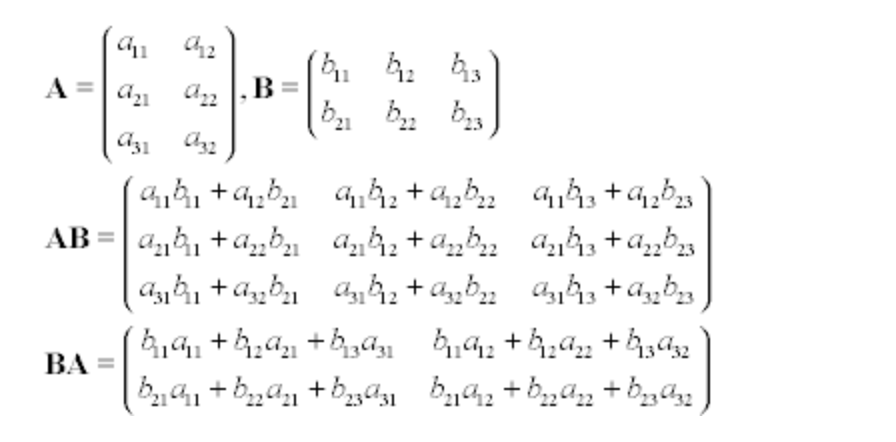
where the number of columns on the left matrix must be equal to the amount of the rows on the matrix on the right.
Some notes that clarified the arithmetic of it, from my wonderful Linear Algebra Professor Dr. Frank Moore: