All-Star Break NBA Computer Ratings Composite


23922293-1Photo Via: Chronicle-Telegram 

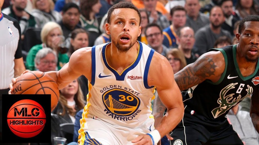
A popular way to look at the strength of teams on this site is through composite ratings. This is an act of compiling an aggregate of differing ratings and combining them into one. This time I will be doing this method for NBA Teams at the all-star break.

The original idea came from Ken Massey’s College Football and College Basketball Computer Composite Ratings, however, he does not publish such ratings for pro sports teams. There are indeed less available computer ratings for Pro Sports Teams than there are for college teams, however, there does exist an ampt amount. I took 25 different NBA Computer Ratings and Rankings and compiled them into one.

The methodology is as follows:

30-(Σ(Ranks)/Number of Ratings)+(Median of Ranks))/2


then I use a way of normalizing dubbed future scaling just to make the Numbers more clear and easy to read. T The future scaling formula forces all values to be between [0, 1], however I multiply it by 100.


Rough Rating Equilvinces: 

95-100: Finals Favorites

90-95: Elite

80-90: Very good but not Elite

70-80: Above Average Playoff Competing Team

60-70: Average Playoff Team

45-60: Borderline Playoff Team/Sub Par Playoff Team

30-45: Below Average NBA Team but Not Horrible

20-30: For Sure Lottery Team

0-20: Awful


(Rating of Team A-Min. Rating in Data Set)/(Max Rating in Data Set-Min Rating in Data Set) * 100

Here are the 25 Different Ratings I used:

  1. NBA W-L%
  2. ESPN BPI
  3. RPI
  4. Sagarin
  5. Massey Ratings
  6. Power Ratings Hoop Index
  7. DRatings
  8. Sonny Moore Ratings
  9. SRS
  10. Fivethirtyeight Full Strength CARMELO
  11. Fivethirtyeight Current CARMELO
  12. Fivethirtyeight Pure Elo
  13. The Power Rank
  14. Numberfire
  15. Team Rankings Predictor
  16. Team Rankings Overall Power Ratings
  17. Compughter Ratings
  18. Talismanred
  19. Dolphin Standard Rankings
  20. Dolphin Improved RPI
  21. Dolphin Predictive
  22. Simmons Ratings
  23. Logan Sports Ratings
  24. Time Travel Sports
  25. Stat Fox

NBA Computer Ratings Composite at the All-Star Break:

  1. Milwaukee Bucks (43-14): 100.00
  2. Golden State Warriors (41-16): 96.65
  3. Toronto Raptors (43-16): 92.94
  4. Oklahoma City Thunder (37-20): 87.35
  5. Denver Nuggets (39-18): 84.07
  6. Boston Celtics (37-21): 79.94
  7. Philadelphia 76ers (37-21): 78.90
  8. Utah Jazz (32-25): 75.96
  9. Indiana Pacers (38-20): 75.47
  10. Portland Trail Blazers (34-23): 72.54
  11. Houston Rockets (33-24): 69.74
  12. San Antonio Spurs (33-26): 60.57
  13. Los Angeles Clippers (32-27): 54.37
  14. Minnesota Timberwolves (27-30): 51.08
  15. New Orleans Pelicans (26-33): 49.06
  16. Los Angeles Lakers (28-29): 42.49
  17. Orlando Magic (27-32): 42.21
  18. Dallas Mavericks (26-31): 41.02
  19. Sacramento Kings (30-27): 40.75
  20. Brooklyn Nets (30-29): 36.97
  21. Miami Heat (26-30): 34.24
  22. Detroit Pistons (26-30): 33.75
  23. Charlotte Hornets (27-30): 26.07
  24. Washington Wizards (24-34): 21.17
  25. Memphis Grizzlies (23-36): 19.57
  26. Atlanta Hawks (19-39): 12.65
  27. Chicago Bulls (14-44): 9.36
  28. New York Knicks (11-47): 3.42
  29. Phoenix Suns (11-48) : 2.80
  30. Cleveland Cavaliers  (12-46): 0.00

Division Ratings:

  1. Northwest: 74.20
  2. Atlantic: 58.43
  3. Southwest: 47.99
  4. Pacific: 47.41
  5. Central: 43.72
  6. Southeast: 27.27

Western Conference: 56.53

Eastern Conference: 43.14


Teams that no one can agree on:

  1. Orlando Magic Std Dev: 4.32 High: #2 Low: 23
  2. Sacramento Kings Std Dev: 3.84 High: #14 Low: #25
  3. New Orleans Pelicans Std Dev: 3.52 High: #11 Low: #22
  4. Los Angeles Lakers Std Dev: 3.40 High: #13 Low: #24
  5. Washington Wizards Std Dev: 2.87 High: #14 Low: #25

Std Dev: Is Standard Deviation, and I am assuming most of you know what this statistic intales, however for those who do not know. It measures the amount of variation in a set of data values. Therefore teams with high standard deviations have individual rankings that differ greatly from one another or their central tendency.



Estimating and Calculating All-Time NFL MVP Shares

10997579_web1_10997579-8348a7b16dde41bc85224ae6be8c9633
Photo Via: Las Vegas Review-Journal

Chiefs quarterback Patrick Mahomes had a sensational MVP season this year, garnering 82% of all the votes. The NFL MVP is a prestigious award with a storied history. Although there are other MVP Awards in the NFL, the AP Award is commonly known as the main one and the most prestigious. The award started in 1957.

In this article, I will be listing players based on their cumulative NFL MVP Shares. What is that you may ask? Well, MVP Shares are pretty simple as it is simply Votes/Max Votes Possible.

For Example, the 2017 MVP Voting was as follows, Tom Brady 40 votes, Todd Gurley 8 votes, and Carson Wentz 2 votes. There were 50 votes total there for Tom Brady had .8 MVP Shares, Todd Gurley had .16 MVP Shares, while Carson Wentz had .04. I calculated these for every MVP race since the implementation of the award in 1957. However, there was some estimation involved for certain years, as the full voting or none at all was not available for a small amount of them. I used https://mvpvoting.wordpress.com/2011-2018/, for my data as they have nearly every MVP Race with the exact voting breakdown.

The estimation was tricky and my method is not perfect, however here is an explanation for how I calculated the shares for the years in which the full data was not available.

1985: The Award voting for Marcus Allen (33 Votes), and Walter Payton (25 votes) was indeed available. However it is known that Roger Craig and Dan Marino both garnered votes, but the exact number is not published. Therefore I used the last available total votes for my calculations. This was 1983, where there were a total of 84 votes. Therefore I calculated Allen’s and Payton’s as usual: 33/84 and 25/84. For the last two, I simply divided the rest evenly between Marino and Craig such that: it was 13/84 for both of them.

1984: 1984 Followed the same adjustments as in 1985. Only the exact votes of Dan Marino (52) and Erick Dickerson (18) were known, but Walter Payton received an unknown # of votes. Therefore I allocated the remaining 14 votes to Payton.

1977 and 1976 both had unknown vote-getters, and I used a total of 84 for both of them.

1975: This was one of the harder ones to estimate as, all we knew was who won the award (Fran Tarkenton), the runner-up (OJ Simpson) and the other players who received votes. Therefore I allocated 84 total votes and based the distribution of these votes on the 1976 finish. Therefore Tarkenton received 41/84, OJ Simpson 19/84, and the rest were allocated evenly.

1971:  1971 had available voting details for the winner Alan Page (16 Votes), Roger Staubach (10), Ottis Taylor (10), Bob Griese (9), Billy Kilmer (4), Boby Lily (1), and Carl Eller (1), However Larry Csonka, Paul Warfield, Len Dawson, John Hadl, John Brodie, and Greg Landry also received votes. Therefore I adjusted the total vote tally from 51 to 57 and allocated one vote to each of the six remaining people.

1970: 1970 had available voting details for the winner John Brodie (33 Votes), George Blanda (27), Alan Page (3), and Fran Tarkenton (3). Nine players also received votes, for the remaining 9 I allocated one each with a new total of 75.

1961: In 1961 we knew that Paul Hornung won the award, and six other players received votes. We also knew the order in which the rest received votes. Therefore I used the distribution from 1968.

1960: There were no voting numbers available for this year however Norm Van Brocklin and Joe Schidmt were co MVP-Winners. Therefore I just allocated shares of .5 to both of them.

With no further ado here is the all-time NFL leaderboard in MVP Win Shares:

Way Too Early 2019 College Football Composite Rankings

justyn-rose-010719-getty-ftrjpg_ryutyckmad2315fsbpqqjfdqi

Photo Via: Sporting News

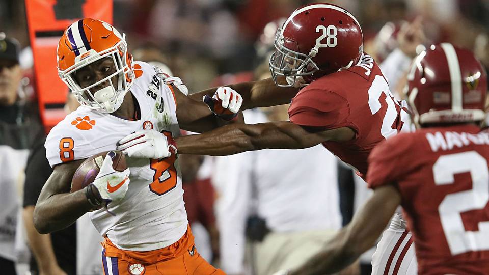
It is everybody’s favorite time of the year; the week after the National Championship Game where loads of sports publications publish their way too early outlooks for the upcoming college football season. Surprisingly Alabama remained #1 on many of the polls despite Clemson’s 44-16 throbbing of them in the Title Game. However Clemson topped them on a slim margin my composite rankings.

I compiled 20 different Way Too Early Top 25’s, and used the method the AP Poll does for their rankings. This means a each #1 place garners a team 25 points, #2 24 points, #3 23 points, and so on until #25 which garners you 1 point.

The 20 Rankings that I used were:

  1. ESPN
  2. 247 Sports
  3. Bleacher Report
  4. NCAA.Com
  5. Sporting News
  6. Athlon Sports
  7. USA Today
  8. Dallas News
  9. Fansided
  10. Al.Com
  11. HeroSports
  12. CFN
  13. My Own Personal Rankings
  14. Sports Illustrated
  15. Orlando Sentinel
  16. ActionNetwork
  17. CBS Sports
  18. HatSports
  19. Saturday Blitz
  20. Yardbreaker

The Way Too Early 2019 Composite Rankings:

Key:

# by Team: Points

(#): First Place Votes

High: Highest Ranking Received

Low: Lowest Ranking Received

  1. Clemson Tigers ACC 491 (11) High: #1 Low: #2
  2. Alabama Crimson Tide SEC 489 (9) High: #1 Low: #2
  3. Georgia Bulldogs SEC 457 High: #3 Low: #4
  4. Ohio State Buckeyes Big 10 432 High: #3 Low: #6
  5. Oklahoma Sooners Big 12 409 High: #4 Low: #12
  6. Texas Longhorns Big 12 378 High: #4 Low: #13
  7. LSU Tigers SEC 359 High: #4 Low: #13
  8. Florida Gators SEC 354 High: #5 Low: #14
  9. Michigan Wolverines Big 10 344 High: #5 Low: #11
  10.  Notre Dame Fighting Irish Ind 337 High: #5 Low: #13
  11. Texas A&M Aggies SEC 291 High: #6 Low: #20
  12. Oregon Ducks PAC 12 285 High: #7 Low: #19
  13. Washington Huskies PAC 12 260 High: #7 Low: #19
  14. Penn State Nittany Lions Big 10 233 High: #10 Low: #19
  15. UCF Golden Knights AAC 193 High: #12 Low: #23
  16. Utah Utes PAC 12 146 High: #14 Low: UR
  17. Wisconsin Badgers Big 10 143 High: 14 Low: #24
  18. Auburn Tigers SEC 134 High: #11 Low: UR
  19. Iowa Hawkeyes Big 10 111 High: #16 Low: UR
  20. Iowa State Cyclones Big 12 104 High: #14 Low: UR
  21. Washington State Cougars PAC 12 86 High: #13 Low: UR
  22. Syracuse Orange ACC 68 High: #12 Low: UR
  23. Missouri Tigers SEC 59 High: #18 Low: UR
  24. Northwestern Wildcats Big 10 47 High: #19 Low: UR
  25. Nebraska Cornhuskers Big 10 45 High: #18 Low: UR

Also Receiving Votes: Army 38, Stanford 33, Kentucky 28, Virginia Tech 27, Mississippi State 26, Michigan State 24, USC 20, OK State 11, Miami 11, Cincinnati 4, Utah State 4, Minnesota 4, TCU 3, Baylor 3, South Carolina 3, Fresno State 3, Houston 2, Boise State 2, Florida State 2, UAB 1

Outtakes from Composite Poll:

-Alabama and Clemson’s World: If the past four years have not made it clear enough, the outlook on the 2019 season shows once again that Nick Saban and Dabo Swinney have their programs in a tier above the rest.

-Loads of Big Games to look forward to in 2019: Many of the Top 15 teams play each other in conference and out of conference next year.

Here are the Top 15 Matchups: #11 Texas A&M @ #2 Clemson, #5 Oklahoma vs. #6 Texas, #6 Texas vs. #7 LSU, #9 Michigan @ #14 Penn State, #9 Michigan vs. #10 Notre Dame, #4 Ohio State @ #9 Michigan, #4 Ohio State vs.  #14 Penn State, #3 Georgia vs. #10 Notre Dame, #12 Oregon @ #13 Washington, #2 Alabama @ #11 Texas A&M, #2 Alabama vs. #7 LSU, #7 LSU vs. #8 Florida, #7 LSU vs. #11 Texas A&M, #3 Georgia vs. #11 Texas A&M, #3 Georgia vs. #8 Florida.

-The Top Programs Remain at the Top: The Top 15 is full of blue blood college football programs, both in a historical sense and recent sense: The Top 15 has combined for 15 National Titles, 29 National Title Game Apps, 65 Conference Titles, 61 AP Top 5 Finishes, 101 AP Top 10 Finishes, 168 AP Top 25 Finishes, 131 10+ Win Years, and 18 Playoff Apps Since 2000.

-Clear Idea for the Top 14 not so much for the rest: Through the compilation of these rankings, it becomes clear that most people think the teams from #1 to #14 are going to be step above the rest going into next year. However after Penn State’s spot at #14, the rankings had great variability regarding who should make up 15-25.  The Average standard deviation for the Top 14 Teams was 1.78 while the average standard deviation for 15-25 was 2.8. That is a clear divergence.


12/10/18 NBA Computer Ratings

maxresdefault-1

Primer on my NBA Computer Ratings:

Like most other ratings of mine, my NBA Ratings follow an Earned Ranking method rather than a predictive ranking method. By this I mean, its goal is to rank teams according to their past performance in the season. Unlike many other earned ranking systems, I do not ignore scoring margin completely.  The ratings that follow give you a look into how good teams have been in the season thus far based on their wins and losses, the strength of teams played, and how dominant they have been.  There are 3 components.


Component 1: W-L%

This is simply (Wins/Total Games Played)


Component #2: SOS

The strength of schedule component is calculated simply:

((2/3 opponent’s W-L%) + (1/3 opponent’s opponent’s W-L%)) * 1.5

The 1.5 coefficient exists in order to assign more importance and deviation in a team’s strength of schedule, as there is naturally not a huge variation in aggregate Opponent’s w-L% in the NBA.


Component #3: Schedule Adjusted Net Rating

The idea of offensive and defensive ratings have become more and more commonplace in the NBA world.  It boils down to points scored per 100 possessions (offensive rating) and points allowed per 100 possessions (defensive rating). I acquire these ratings from basketballreference.com. The net rating (Off Rat-Def Rating) is calculated then using an iterative process is adjusted for the average ratings of the team’s played.

Here are the formulas commonly used for offensive and defensive rating:

Offensive Rating: 100 x Pts / (0.5 * ((Tm FGA + 0.4 * Tm FTA – 1.07 * (Tm ORB / (Tm ORB + Opp DRB)) * (Tm FGA – Tm FG) + Tm TOV) + (Opp FGA + 0.4 * Opp FTA – 1.07 * (Opp ORB / (Opp ORB + Tm DRB)) * (Opp FGA – Opp FG) + Opp TOV)))

Defensive Rating: Follows the same formula but instead of 100 x Pts its 100 x Opponent’s points.

The ratings are calculated then their opponent’s average net rating is added or subtracted to it, numerous times until they converge within an iterative process.

Comp #3 Formula= (Adjusted Net Rating) * .8

The .8 is to account for the great variation in net ratings within the league as well as to prevent a team who is running the score up to gain a higher rating.


These 3 components are then averaged and multiplied by a 100 to give the rating.


12/9/18 NBA Power Ratings:

  1. Toronto Raptors 21-7 51.70
  2. Milwaukee Bucks 17-8 51.50
  3. Denver Nuggets 17-9 48.78
  4. Golden State Warriors 18-9 48.20
  5. Los Angeles Clippers 16-9 47.90
  6. Philadelphia 76ers 18-9 47.33
  7. Oklahoma City Thunder 16-8 46.58
  8. Portland Trail Blazers 15-11 46.14
  9. Boston Celtics 15-10 46.06
  10. Memphis Grizzlies 15-10 45.92
  11. Los Angeles Lakers 16-10 45.64
  12. Indiana Pacers 16-10 44.90
  13. Utah Jazz 13-14 43.16
  14. Sacramento Kings 13-12 43.10
  15. Minnesota Timberwolves 13-13 42.77
  16. Dallas Mavericks 13-11 42.56
  17. New Orleans Pelicans: 14-14 42.52
  18. Charlotte Hornets: 13-13 41.57
  19. Detroit Pistons: 13-11 41.25
  20. San Antonio Spurs 13-14 40.98
  21. Orlando Magic 12-14 40.80
  22. Houston Rockets 11-14 3.39
  23. Miami Heat 11-14 37.57
  24. Washington Wizards 11-15 37.39
  25. Brooklyn Nets  10-18 35.67
  26. New York Knicks 8-20 32.68
  27. Cleveland Cavaliers 6-20 30.30
  28. Atlanta Hawks 6-20 30.16
  29. Chicago Bulls 6-21 29.75
  30. Phoenix Suns 4-22  29.22


NFL Week 11 Computer Composite Ratings

la-sp-rams-vs-saints-20181104-pictures-012-1.jpg

Photo Via: LA Times

There are numerous different NFL Rating systems and computer ratings. The rankings differ far and wide, from ratings that solely focus on how much you a beat team by, and other rankings who don’t factor margin of victory at all. I took a composite of 33 different NFL Ratings that I could find on the internet, to create power ratings for Week 11.

To calculate the composite I averaged the ratings of each team to get the mean, then I took the median of each team’s ratings. I then averaged these two together. I did not solely use the arithmetic mean due to the fact it can be influenced by outliers while the median is not.

I then used a normalization statistical method called future scaling. I have used future scaling in previous articles, such as my Power Ratings of International Soccer Countries going into the World Cup. The scaling here is done for more arbitrary reasons to give the team’s a rating from 0-100.  Therefore the formula for the composite is as follows:

(32-((∑(Team Ratings)/33)+Median*)/2))/(32-1))*100

*Median= (Rank the Values from highest to lowest, the middle number is the median, in this case, it was the 17th rating)


Rankings included:

  1. NFL W-L%
  2. PowerRatings.com
  3. Roundtable Ratings
  4. Burdorf Ratings
  5. Stat Fox
  6. Time Travel Sports
  7. Golden
  8. Sagarin
  9. Jelly Juke
  10. Team Rankings Predictor
  11. Team Rankings Overall
  12. Dolphin Ratings
  13. Dolphin Improved RPI
  14. Compughter NFL Ratings
  15. Jeff Self Ratings
  16. Massey NFL Ratings
  17. D Ratings
  18. Coffey Ratings
  19. 538 Elo
  20. ESPN FPI
  21. Transitive W-L%*(Basic Rating that I made, formula in article)
  22. Sports Reference SRS
  23. Performance Z Ratings
  24. Pi Ratings
  25. Sonny Moore Power Ratings
  26. Nutshell Ratings
  27. Bassett Ratings
  28. Kalin Ratings
  29. Brian Simmons Ratings
  30. Jeff Bihl Rankings
  31. Argh Power Ratings
  32. Round Robin W-L%
  33. PFF Elo

*Transitive W-L% is a simple ranking system to rate teams based on who they have beat and who they have lost to. The result of the game (Win or Loss) and the opponent’s Wins and losses are the only things that matter.

Formula: (Cumulative Wins of Team’s Beat)/(Cumulative Wins of Team’s Beat + Cumulative Losses of Teams lost to)

E.G.: Team A beats, Team B(1-2), Team C(2-1), and loses to Team D(1-2).  They have 3 transitive wins and 2 transitive losses. Their rating is 3/5=.600

(W-L)


Week 11 NFL Composite Power Ratings:

  1. New Orleans Saints (99.02) NFC South High: #1 Low: #4
  2. Kansas City Chiefs (96.43) AFC West High: #1 Low: #4
  3. Los Angeles Rams (93.50) NFC West High: #1 Low: #12
  4. Pittsburgh Steelers (90.76) AFC North High: #2 Low: #7
  5. Los Angeles Chargers (86.31) AFC West High: #3 Low: #8
  6. New England Patriots (82.94) AFC East High: #4 Low: #12
  7. Carolina Panthers (75.22) NFC South High: #6 Low: #17
  8. Chicago Bears (74.29) NFC North High: #5 Low: #17
  9. Baltimore Ravens (70.43) AFC North High: #5 Low: #19
  10. Houston Texans (65.93) AFC South High: #7 Low: #20
  11. Minnesota Vikings (65.44) NFC North High: #5 Low: #16
  12. Tennesee Titans (64.81) AFC South High: #3 Low: #18
  13. Seattle Seahawks (61.39) NFC West High: #5 Low: #19
  14. Washington Redskins (58.06) NFC East High: #7 Low: #22
  15. Green Bay Packers (54.69) NFC North High: #9 Low: #19
  16. Atlanta Falcons (52.00) NFC South High: #11 Low: #21
  17. Philadelphia Eagles (49.36) NFC East High: #5 Low: #23
  18. Dallas Cowboys (48.58) NFC East High: #9 Low: #21
  19. Cincinnati Bengals (45.45) AFC North High: #5 Low: #29
  20. Indianapolis Colts (39.88) AFC South High: #8 Low: #24
  21. Denver Broncos (33.72) AFC West High: #13 Low: #27
  22. Cleveland Browns (31.43) AFC North High: #18 Low: #31
  23. Tampa Bay Buccaneers (28.45) NFC South High: #17 Low: #29
  24. Jacksonville Jaguars (28.40) AFC South High: #18 Low: #28
  25. Detroit Lions (23.70) NFC North High: #18 Low: #27
  26. Miami Dolphins (21.75) AFC East High: #14 Low: #30
  27. New York Giants (16.52) NFC East High: #20 Low: #32
  28. Buffalo Bills (13.54) AFC East High: #23 Low: #32
  29. San Francisco 49ers (12.56) NFC West High: #23 Low: #32
  30. New York Jets (9.29) AFC East High: #25 Low: #31
  31. Arizona Cardinals  (7.14) NFC West High: #24 Low: #32
  32. Oakland Raiders (0.24) AFC West High: #31 Low: #32


Introducing a New Rating System: Time Margin Matrix (TIMEMAT)

Screenshot 2018-11-04 16.37.38.png

Firstly i would like to apologize for the lack of content the past month, I have been working on a lot of academic related material, and been constructing this system. This rating system is the most mathematically complex one I have constructed to this date, therefore I welcome any questions regarding it. It actually involved two metrics, one is a new way to look at margin of victory, and the other takes a lot from Ken Massey’s esteemed rating system. I will also be using this system for College Football teams currently, however it can be used for practically any sport!

Part 1: Time Adjusted Margin(TAM)
The most contemporary way to look at how dominant a team is in any sport, is the Margin of Victory. Which is simply subtracting the opponent’s points from the team’s points. It is a controversial metric in the realm of advanced ratings, as it can overvalued teams that run up the score. However, I am of the opinion, that it is a necessary aspect. If Team B and C both beat Team A, but team B wins by 28 while Team C wins by 3, those wins should not be counted the same.

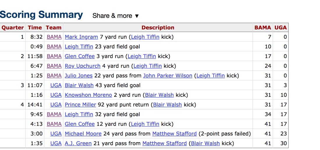
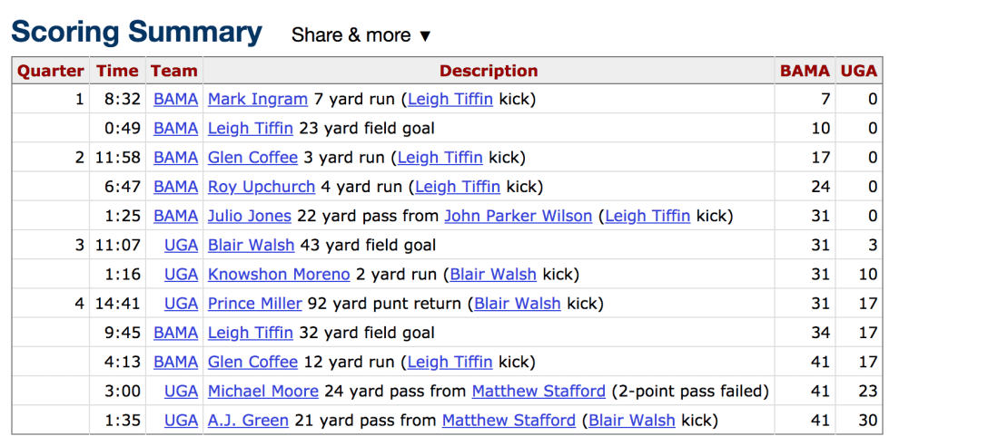
Another flaw of basic margin of victory is that it can be misleading. Teams that go up by 3 or 4 scores early, will often sub in their second and third strings which allows other teams to score garbage time touchdowns. A prime example of this would be 2008 Alabama’s showdown vs. #3 Georgia. The Final score was 41-30, which gives the impression Alabama pulled away at the end, however that was simply not the case. The Crimson Tide went up 31-0 in the first half and were up 41-17 with four minutes left in the fourth.

On the other end a highly contested matchup, with the opposing teams going back and forth, can seem lopsided when just looking at the final score. A prime example, also coming from Alabama, was their 37-21 win over Texas in the 2009 season’s national title game. Star quarterback Colt McCoy went down for the Longhorns early, and despite this, the score was 24-21 prior to the 2: 00-minute mark in the last quarter. Fluke instances or team’s trying to put the game away can make a back and forth contest seem lopsided.

This is why I created Time Adjusted Margin, which is calculated based on the following:
(60-(Final time in the game when team went up by more than 8 Points)

The essence is not entirely clear just based on the formula, therefore I will use some examples.

Screenshot 2018-11-04 15.12.51.png

The raw, time-adjusted margin would be 46, because Alabama went up 10-0 at the 1 minute mark in the first, with 46 minutes left in the game. An important thing to remember is that, if Georgia had gotten the score to 31-24 at some point in the game, it would have been different. The metric is based on the time the team went up by more than one possession, and never relinquished that 1+ possession lead for the entirety of the game. While Georgia would have had a margin of -46.

Screenshot 2018-11-04 15.06.21

The raw, time-adjusted margin in this game would have been 2 because Alabama went up by 10 at the 2:01 mark in the fourth, not 30 despite the fact they went up by 11 at the 29 second mark in the second quarter.

Some Adjustments that should be noted:
-Games that finish within one score are assigned a rating of 5, to still provide emphasis on winning, even if it came in the last minutes. Also teams who go up by more than one possession within the 5 minute mark in the fourth, are also assigned a 5.
there is a home/away adjustment which is +/- 3.43, this is based on the least squares regression equation of, and the 2.5 standard home-field advantage usually used by odds makers:

y=1.31x+0.15
x being the Time margin with y being the margin of victory.

Part 2: TIMEMAT

This system is based on Kenneth Massey’s Matrix system in which he uses the linear algebra least squares equation of:
Screenshot 2018-11-04 15.24.36.png

To fully understand the mathematics behind this, one should most likely have some sort of experience in Linear Algebra. However I will try my best to explain it in such way, where one will get a decent idea of it no matter their background. The whole point of this site, is to remove the ambiguity involving advanced metrics, and give readers insight into what they are actually seeing when they see metrics thrown around. If you are intrigued by this I would highly recommend the book: The Science of Rating and Ranking Who’s #1 by Amy N. Langville and Carl D. Meyer. They do a great job at explaining the system that Massey uses!

When looking at larger sample sizes, it is nearly impossible to look at matrices just as a system of linear equations, therefore I will use the games played between Texas, Texas Tech, Oklahoma and Oklahoma State in the 2008 Big 12 South.

The Games resulted in the following:
Texas beating Oklahoma in a neutral site TAM: 5.0
Oklahoma beating Texas Tech at Home TAM: 40.57
Oklahoma beating OK State on the Road TAM: 10.43
Texas beating OK State at home TAM: 1.57
Texas Tech beating Texas at home TAM: 1.57
Texas Tech beating OK State at home TAM: 27.57

You start off with a Matrix m (games played) x n (# of teams) matrix, X. You are trying to solve for the system Xr=y where x is a team, r are the ratings you are trying to calculate, and y is the list of Time Adjusted Margins of each game. (X1=Oklahoma, X2=Texas, X3=Texas Tech, X4=OK State)

OU vs. Texas: -1×1+1×2+0x3+0x4=5
OU vs. Texas Tech: 1×1+0x2-1×3+0x4=40.57
OU vs. OK State: 1×1+0x2+0x3-1×4=1.57
Texas vs. OK State: 0x1+1×2+0x3-1×4=1.57
Texas Tech vs. Texas: 0x1-1×2+1×3+0x4=1.57
Texas Tech vs. OK State: 0x1+0x2+1×3-1×4=27.57

If you could not tell already, a team that wins the game gets a 1 and the team that loses gets a -1, and a team not involved in that particular match-up has a coefficent of 0.

You then transpose this where the rows become the columns, and vice versa, which looks like
OU:-1w1+1W2+1w3+0w4+0w5+0w6
Texas: 1w1+0w2+0w3+1w4+-1w5+0w6
Texas Tech: 1w1+0w2+0w3+1w4-1w5+0w6
OK State: 0w1+0w2-1w3-1w4+0w5-1w6

the w’s here are each game played, which is why some teams have a coefficient for each w while others don’t because obviously Texas Tech was not involved in the Texas Oklahoma Game. Then I use matrix multiplication to multiply this system by the previous system and set it equal to XT times the Y Vector which simply becomes the cumulative Time Margins of each team, which turns into :

3×1-1×2-1×3-1×4=46
-1×1+3×2-1×3-1×4=5
-1×1-1×2+3×3-1×4=-11.43
-1×1-1×2-1×3-1×4=-39.57

It is hard to see how this equation has any merit without understanding linear algebra. In summation, it simply creates n x n square matrix, that builds dependence within it. In the sense that the matrix inherently accounts for such things, as the strength of schedule. The process is trying to simply find the closest set of ratings that accounts for the given data of a team beating certain team given a certain time margin.

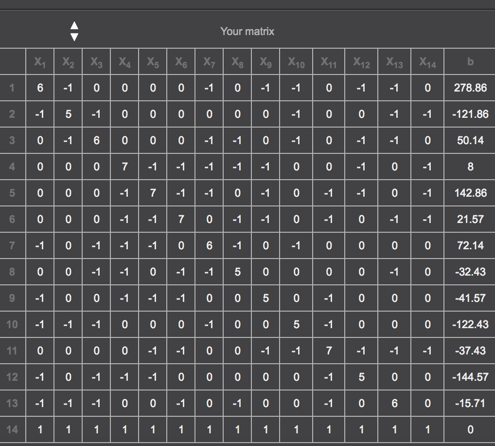
Massey uses an adjustment to make the matrix invertible, and something that in a way scales it by making one of the lines all 1s, and the corresponding entry in the Y vector, to Zero. The mathematics behind this are based in the fact, that no matter how the schedule works out (even if they play a team multiple times), the sum of the rows is 0. This means that the all ones vector is in the null space of the matrix, and maps the system to the zero vector. If one replaces an arbitrary row of the coefficents with all ones, and a zero on the right. This set of ones, is no longer in the solution set as the right side gives M (# of teams and not zero). The Matrix’s other entries are based on the other team’s results therefore one can replace any row and still yield the same results:

Solving the system using Gaus-Jordan Elimination:
(3×1-1×2-1×3-1×4)*R1=46
(-1×1+3×2-1×3-1×4)*R2=5
(-1×1-1×2+3×3-1×4)*R3=-11.43
(1×1+1×2+1×3+1×4)*R4=0

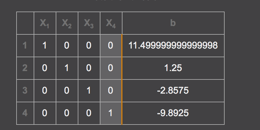
yields these ratings:
Screenshot 2018-11-04 16.10.09.png

1. Oklahoma 11.50
2. Texas 1.25
3. Texas Tech -2.86
4. OK State: -9.89

Keep in mind, this small sample size is based simply on the games played between the two teams, and the ratings would be different if you expanded it to the entirety of the season.

These ratings can be used to predict the outcome of games, if Oklahoma had played Texas Again, the metric would predict Oklahoma to go up by more than 1 poss. at 10 minute mark in the fourth quarter since (11.50-1.25-10.25), which translates to a pretty close game.

I also calculated the ratings for the SEC teams based solely on their conference games this year:

which gave the results:
Screenshot 2018-11-04 21.22.12.png

The order of the teams were as followed in the matrix: Alabama, Ark, Auburn, Florida, Georgia, Kentucky, LSU, Miss State, Ole Miss, Mizzou, SC, Tennessee, TAMU, Vandy.

1. Alabama 39.8
2. LSU 18.83
3. Georgia 18.33
4. Kentucky 2.79
5. Mizzou 2.48
6. Florida 2.43
7. Auburn 0.99
8. TAMU -1.10
9. Miss State -1.68
10. South Carolina -13.25
11. Vanderbilt -13.25
12. Vols -18.48
13. Ole Miss -19.01
14. Arkansas -22.87

In summation: This rating system solves the equation in the closest way possible: of ra-rb=t, where RA is the rating of Team A, and RB is the rating of team B, and T is the time margin.

The system is only useful when comparing teams within comparable samples. If were to do this for the Mountain West Conference, a good team like Fresno State would possibly have a higher rating than a better sec team like Georgia. This is easily solvable, by just putting data from the whole season, conference and nonconference play. I will be computing this sometime soon, once I find the most efficient way to aquire the data.

Here are some facts and properties of linear algebra that build one’s understanding of the system:

What is a matrix?:Screenshot 2018-11-04 16.24.24.png

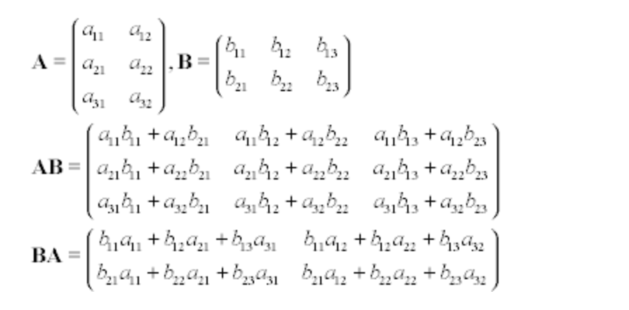
Matrix Multiplication: Screenshot 2018-11-04 16.22.27.png

where the number of columns on the left matrix must be equal to the amount of the rows on the matrix on the right.

Some notes that clarified the arithmetic of it, from my wonderful Linear Algebra Professor Dr. Frank Moore:
Screenshot 2018-11-04 16.27.43.png

Stat of the Week #3: Looking at the Biggest NFL Upsets Since 2000

NFL: Minnesota Vikings at Buffalo Bills
Photo Via: USA Today
The NFL is notorious for being a parity-filled league primarily due to its’ strict salary cap rules and relatively low salaries for top tier players (compared to other leagues). This parity is shown in betting lines, as game spreads seldomly exceed 20.0, while this is a quite common occurrence in college football.

I used Sports Reference to compile the biggest NFL upsets since 2000 according to the spread. This data is up to Week 3 of the 2018 NFL Season.
*= Theres more than 50 games here just because there were several games with a 10.5 point spread

Top 50* Upsets Since 2000:
1. Bills 27 @ Vikings 6 2018 Week 3 Line: 16.5 +/-: 37.5
2. Raiders 27 @ Steelers 24 2009 Week 13 Line: 15.0
+/-: 18.0
3T. Cardinals 21 @ Eagles 20 2001 Week 4 Line: 14.5 +/-: 15.5
3T. Vikings 24 @ Eagles 14 2010 Week 16 Line: 14.5 +/-: 24.5
5T. Patriots 20 vs. Rams 17 2001 Super Bowl Line: 14.0 +/-: 17.0
5T. Texans 24 @ Steelers 6 2002 Week 14 Line: 14.0 +/-: 32.0
5T. Texans 21 @ Dolphins 20 2003 Week 1 Line: 14.0 +/-: 15.0
5T. Lions 39 @ Cowboys 31 2006 Week 17 Line: 14.0 +/-: 22.0
5T. Raiders 20 @ Broncos 19 2009 Week 15 Line: 14.0 +/-: 15.0
5T. Buccaneers 20 @ Saints 17 2009 Week 16 Line: 14.0 +/-: 17.0
5T. Raiders 13 vs. Eagles 9 2009 Week 6 Line: 14.0 +/-: 18.0
5T. Rams 31 vs. Saints 21 2011 Week 8 Line: 14.0 +/-: 24.0
5T. Dolphins 20 @ Falcons 17 2017 Week 6 Line: 14.0 +/-: 17.0
14T. Saints 31 @ Rams 24 2000 Week 13 Line: 13.5 +/-: 20.5
14T. Panthers 27 @ Rams 24 2000 Week 10 Line: 13.5 +/-: 16.5
14T. Dolphins 23 @ Chargers 21 2005 Week 14 Line: 13.5 +/-: 15.5
14T. Dolphins 31 @ Bears 13 2006 Week 9 Line: 13.5 +/-: 31.5
14T. Rams 19 @ Redskins 17 2008 Week 6 Line: 13.5 +/-: 15.5
14T. Cardinals 20 @ Patriots 18 2012 Week 2 Line: 13.5 +/-: 15.5
14T. Giants 23 @ Broncos 10 2017 Week 6 Line: 13.5 +/-: 26.5
21T. Cardinals 34 @ Raiders 31 2001 Week 12 Line: 13.0 +/-: 16.0
21T. Bills 37 @ Bengals 27 2005 Week 16 Line: 13.0 +/-: 23.0
21T. Titans 31 @ Eagles 13 2006 Week 11 Line: 13.0 +/-: 31.0
21T. Raiders 28 @ Chargers 13 2010 Week 13 Line: 13.0 +/-: 28.0
21T. Cardinals 21 @ Eagles 17 2011 Week 10 Line: 13.0 +/-: 17.0
26T. Rams 20 @ Cowboys 10 2006 Week 17 Line: 12.5 +/-: 22.5
26T. Giants 17 vs. Patriots 14 2007 Super Bowl Line: 12.5 +/-: 15.5
26T. Dolphins 38 @ Patriots 13 2008 Week 3 Line: 12.5 +/-: 37.5
26T. Browns 30 @ Saints 17 2010 Week 7 Line: 12.5 +/-: 25.5
26T. Cowboys 33 @ Giants 20 2010 Week 10 Line: 12.5 +/-: 25.5
31T. Saints 34 @ Rams 31 2001 Week 7 Line: 12.0 +/-: 15.0
31T. Giants 26 @ Rams 21 2002 Week 2 Line: 12.0 +/-: 17.0
31T. Cowboys 13 @ Rams 10 2002 Week 4 Line: 12.0 +/-: 15.0
31T. Lions 30 vs. Rams 10 2003 Week 17 Line: 12.0 +/-: 32.0
31T. Titans 25 @ Redskins 22 2006 Week 6 Line: 12.0 +/-: 15.0
31T. Chiefs 30 @ Chargers 16 2007 Week 4 Line: 12.0 +/-: 26.0
31T. Rams 23 @ Seahawks 17 2015 Week 16 Line: 12.0 +/-: 18.0
38T. Patriots 44 vs. Colts 13 2001 Week 3 Line: 11.5 +/-: 42.5
38T. Falcons 27 @ Giants 7 2003 Week 10 Line: 11.5 +/-: 31.5
38T. Raiders 25 @ Broncos 24 2004 Week 12 Line: 11.5 +/-: 12.5
38T. 49ers 15 vs. Buccaneers 10 2005 Week 8 Line: 11.5 +/-: 16.5
38T. Chiefs 27 vs. Steelers 24 2009 Week 11 Line: 11.5 +/-: 14.5
38T. Chiefs 19 vs. Packers 14 2011 Week 15 Line: 11.5 +/-: 16.5
38T. Jaguars 29 @ Titans 27 2013 Week 10 Line: 11.5 +/-: 13.5
45T. Steelers 24 @ Jaguars 13 2000 Week 5 Line: 11.0 +/-: 22.0
45T. Texans 21 @ Jaguars 19 2002 Week 8 Line: 11.0 +/-: 13.0
45T. Chargers 28 @ Colts 24 2007 Divisional Round Line: 11.0 +/-: 15.0
48T. Bengals 17 vs. Jaguars 14 2000 Week 16 Line: 10.5 +/-: 13.5
48T. Cowboys 27 @ Redskins 21 2000 Week 3 Line: 10.5 +/-: 16.5
48T. Patriots 38 @ Colts 17 2000 Week 6 Line: 10.5 +/-: 31.5
48T. Bears 19 @ Broncos 10 2003 Week 12 Line: 10.5 +/-: 19.5
48T. Jets 17 @ Patriots 14 2006 Week 10 Line: 10.5 +/-: 13.5
48T. Texans 13 @ Jaguars 10 2006 Week 10 Line: 10.5 +/-: 13.5
48T. 49ers 37 @ Cardinals 31 2007 Week 10 Line: 10.5 +/-: 16.5
48T. Rams 37 @ Saints 29 2007 Week 10 Line: 10.5 +/-: 18.5
48T. Raiders 31 @ Buccaneers 24 2008 Week 17 Line: 10.5 +/-: 17.5
48T. Jaguars 12 vs. Ravens 7 2011 Week 7 Line: 10.5 +/-: 15.5
48T. Raiders 28 @ Texans 23 2013 Week 11 Line: 10.5 +/-: 15.5
48T. Jets 30 @ Falcons 28 2013 Week 5 Line: 10.5 +/-: 12.5
48T. Rams 13 @ 49ers 10 2014 Week 9 Line: 10.5 +/-: 13.5
48T. Lions 18 @ Packers 16 2015 Week 10 Line: 10.5 +/-: 12.5
48T. Texans 10 @ Bengals 6 2015 Week 10 Line: 10.5 +/-: 14.5
48T. Dolphins 27 vs. Patriots 20 2017 Week 14 Line: 10.5 +/-: 17.5

Takeaways:
-The Greatest Show on Turf or The Most Upset Prone team on Turf?: The Rams from 2000-2003 had an insane total of 7 different games in which they were a 10.5+ Point Favorite and lost. The most notable of which was their loss as a 14 point favorite in the 2001 Super Bowl against the Tom Brady led Patriots.
-Rams and Raiders were the king of being underdogs: Despite my previous point the Rams had the 2nd most upset wins since 2000 of more than a 10.5 point spread. They had six such instances. The top team were the Raiders with seven . upsets.
=The Patriots started out as underdogs: The Patriots have dominated the NFL since the turn of the century with 5 super bowl wins. However they had 3 different big upsets in their 2001 year, two of which were massive blowout wins vs. The Colts. Their week 3 31 point win was the biggest margin of any game on the list.

Random Stat of the Week #2: Best College Basketball Programs of the 2010s

villanova-vs-kansas-all-time-history.jpg

Photo Via: SI 

This past year the AP Poll ranked the best college football programs based on an aggregate of final AP Poll rankings, giving 25 points to each #1 finish, 24 points to each #2 finish, and so on until  1 point for each #25 finish. They also ranked the best programs of each decade using the same method.

This inspired me to do the same for the current decade in College Basketball. There is no Final AP Poll in College Basketball, however there is a Final Coaches Poll. I used the same method to rank the best programs since 2010 (The Season where Duke Beat Butler). This is not a perfect method of ranking the best programs especially since the Final Coaches Poll is especially skewed by the NCAA Tournament. An example of this is Loyola being ranked higher in the final coaches poll than Cincinnati last year. With that being said it is usually a good indicator when it comes to combing a teams regular season performance with their tournament results in a year.

Best Programs:

1. Kansas Jayhawks: 173
2. Kentucky Wildcats: 156
3. Duke Blue Devils: 155
4. Michigan State Spartans: 125
5. UNC Tar Heels: 118
6. Villanova Wildcats: 109
7. Louisville Cardinals: 96
8. Arizona Wildcats: 95
8. Syracuse Orange: 95
10. Wisconsin Badgers: 90
11. Florida Gators: 89
12. Ohio State Buckeyes: 84
13. Gonzaga Bulldogs: 82
14. Michigan Wolverines: 81
15. Virginia Cavaliers: 76
16. West Virginia Mountaineers: 71
17. Baylor Bears: 63
18. Wichita State Shockers: 62
19. Xavier Musketeers: 59
20. Purdue Boiler Makers: 58
20. Butler Bulldogs: 58
22. Oregon Ducks: 55
23. UCONN Huskies: 50
24. Indiana Hoosiers: 50
25. Notre Dame Fighting Irish: 49

Takeaways:

-The Jayhawks are Great at being very good: Despite not having a single national title this decade, Kansas ranked #1 by a wide margin. Kansas and Duke were the only teams to finish in the Top 25 each season. With the Jayhawks having 6 finishes of #6 or higher.

-Villanova is the king of the second half of the decade: Despite having 3 seasons in a row without finishing in the Top 25 the Wildcats still found a way to be #6.

-Familiar Faces at the Top: Many of the programs that have been dominating the College Basketball scene for decades, are in the Top 10. The Top 10 has a combined 32 titles between them.

-The strange case of UCONN: UCONN is tied with Villanova & Duke for the most national titles this past decade, but has half and a third of the points of the other two powers. This is because the only two times UCONN has finished in the Top 25, they finished #1. They are by far the most inconsistent team this decade, as they have had as many sub .500 seasons as national title seasons.


Random Stat of the Week #1: Most Wins over Teams Ranked in Final AP CFB Poll Since 2010

michigan-notre-dame
Photo via: USA Today

Random stat of the week is a bi-weekly article that will showcase a random statistic. Pretty self explanatory right? The articles however are not subjugated to timely events. In other words the stats may or may not be related to events happening in the world of sports at the time. Also the articles will not only be a single stat, they can be a list of them. This is the case for my the first entry in the series which is a leaderboard of Wins over Final AP Top 25 Teams Since 2010. Stats regarding wins over Top 5, Top 10, Top 25, are widely available, however they are usually based on the Ranks of teams when they were played. My article is based on the Final AP Rankings, which I think is a much better indicator of quality wins.

At the end of the article, I will list some takeaways. Things I found interesting or notable in my compilation of the statistic.

Takeaways:
-Alabama is as dominating as expected. Winning the most games against the toughest competitions. Having the most wins in most of the categories by a fairly large margin. Having 4 more than the next best in Top 5 Wins, one more in Top 10 Wins, 8 more in Top 15 and Top 25.
-Clemsoning is long gone. The idea of Clemson choking against top tier opponents, is a tradition no more. Despite not gaining respect on the national scene until the past three years, Clemson has a myriad of top tier wins. Coming in second for most Top 25 Wins.
-SEC dominance is not a myth. At least half of the Top 10 in Each Category of Wins were from the SEC.
-South Carolina has a niche for beating good teams. Despite going 25-26 since the start of the Playoff Era, the Gamecocks have 2 Top 5 Wins, 6 Top 10 Wins, 8 Top 15, and 17 Top 25 Wins. Most of these came from their peak years from 2010-2013.
-Michigan has had an up and down stretch since 2010, and have no top five wins to show, Iowa, Ole Miss, Northwestern, Houston, Pitt, Syracuse, among many others have had Top 5 Wins inn that same time span.

Predicting League Tables for The Big 5 Soccer Leagues


5b6aa9edc7e8b_Rashford


The best clubs in the world will be kicking off league play within the next three weeks, with the big 5 Leagues kicking off as follows:

Eng. Premier League: Aug 10

French Ligue 1: Aug 10

Italian Serie A: Aug 18

German Bundesliga: Aug 24

Spanish La Liga: Aug 17

With this comes much anticipation and a plethora of storylines such as: Cristiano Ronaldo debuting with Juventus, Real Madrid’s Post Ronaldo Era, Will Anybody be able to stop Man City?, among others.

I used normalization and a composite of computer ratings to rate the World Cup Teams heading into the tournament, and I am using a similar methodology in projecting the league tables for the top five leagues. These ratings rate teams in comparison within teams in their own league, hence the reasons why teams like Schalke will have a higher rating than teams like Chelsea or Arsenal. The premier league is a tougher league than the Bundesliga which makes it so the 2nd best team in the German League could have a higher rating than the third or fourth best teams in the Premier League. Therefor comparing the ratings of the teams across different leagues is not advised.

Here is a brief summary of my computations:

I first made a composite of five different computer ratings ranking the teams in each of their leagues, then I added two other metrics from Transfermarkt.com which assigns money values to players and teams based on their performances and other facets. I adjusted these ratings with outlier eliminating, and future scaling normalization.

The ratings I used were:

538 Soccer Power Index

Football Database  Elo Based Rankings

Clubelo.com’s European Football Club Elo Rankings

Massey Soccer Computer Ratings

Euro Club Index Ratings

Transfer Markt Total Value

Transfer Market Average Value

Certain ratings did not have data for teams recently promoted into the league, for those recently promoted teams I rated them behind teams that had ratings and then ranked them based on their finish in the second league table within the previous year.

One drawback from these ratings is that they don’t fully adjust for recently acquired transfers or the exit of their own players. This is why I added transfermarkt values.

Max= Max Ranking from composite
Min= Min Rating from composite

Teams with the same composite ratings are ranked based on the following tie breakers:
1. Max Rating
2. Finish in Previous Year’s Table

Power Ratings for the Big 5 Leagues:


English Premier League:

1. Manchester City: 100.00
Max: #1 Min: #1

2. Liverpool: 90.23
Max: #2 Min: #4

3. Tottenham: 89.85
Max: #2 Min: #5

4. Manchester United: 83.83
Max: #3 Min: #6

5. Chelsea: 79.70
Max: #2 Min: #6

6. Arsenal: 74.81
Max: #4 Min: #6

7. Leicester City: 62.41
Max: #7 Min: #10

8. Everton: 62.03
Max: #7 Min: #11

9. Crystal Palace: 56.77
Max: #7 Min: #12

10. Southampton: 48.50
Max: #9 Min: #15

11. West Ham United: 46.24
Max: #8 Min: #15

12. Burnley: 42.86
Max: #9 Min: #15

13. Newcastle United: 34.59
Max: #9 Min: #15

14. AFC Bournemouth: 30.08
Max: #12 Min: #17

15. Brighton & Hove Albion: 25.94
Max: #12 Min: #18

16. Fullham: 25.19
Max: #7 Min: #18

17. Watford: 18.42
Max: #12 Min: #20

18. Wolverhampton: 13.16
Max: #10 Min: #19

19. Huddersfield Town: 5.26
Max: #17 Min: #20

20. Cardiff City: 2.26
Max: #16 Min: #20


Spanish La Liga:

1. Barcelona: 99.25
Max: #1 Min: #2

2. Real Madrid: 95.11
Max: #1 Min: #3

3. Atletico Madrid: 89.85
Max: #2 Min: #3

4. Valencia: 83.46
Max: #4 Min: #5

5. Sevilla: 77.82
Max: #4 Min: #7

6. Villarreal: 72.93
Max: #5 Min: #9

7. Real Sociedad: 62.78
Max: #4 Min: #12

8. Espanyol: 59.77
Max: #7 Min: #12

9. Real Betis: 53.76
Max: #7 Min: #11

10. Getafe: 46.62
Max: #8 Min: #15

11. Celta Vigo: 45.86
Max: #7 Min: #13

12. Eibar: 44.36
Max: #7 Min: #17

13. Athletic Bilbao: 40.98
Max: #6 Min: #15

14. Alaves: 36.84
Max: #8 Min: #16

15. Girona: 27.44
Max: #11 Min: #16

16. Levante: 26.69
Max: #13 Min: #17

17. Leganes: 18.05
Max: #14 Min: #18

18. Rayo Vallecano: 9.40
Max: #17 Min: #20

19. Valladolid: 4.89
Max: #18 Min: #20

20. Huesca: 4.51
Max: #18 Min: #20


Italian Serie A:  

1. Juventus: 100.00
Max: #1 Min: #1

2. Napoli: 93.61
Max: #2 Min: #3

3. Roma: 88.72
Max: #2 Min: #5

4. Inter Milan: 84.96
Max: #2 Min: #5

5. Lazio: 79.32
Max: #4 Min: #6

6. AC Milan: 74.06
Max: #4 Min: #7

7. Atalanta: 68.42
Max: #6 Min: #9

8. AFC Fiorentina: 63.16
Max: #7 Min: #9

9. Torino: 59.02
Max: #8 Min: #9

10. Sampdoria: 51.50
Max: #10 Min: #11

11. Sassuolo: 47.37
Max: #10 Min: #12

12. Genoa: 37.22
Max: #12 Min: #15

13. Udinese: 30.83
Max: #13 Min: #16

14. Cagliari: 27.07
Max: #11 Min: #!7

15. Chievo: 22.56
Max: #12 Min: #18

16. SPAL: 22.56
Max: #12 Min: #18

17. Bologna: 21.05
Max: #14 Min: #18

18. Empoli: 14.66
Max: #12 Min: #19

19. Frosinone: 5.26
Max: #17 Min: #20

20. Parma: 1.50
Max: #18 Min: #20


German Bundesliga:

1. Bayern Munich: 100.00
Max: #1 Min: #1

2. Borussia Dortmund: 88.66
Max: #2 Min: #4

3. Schalke 04: 86.55
Max: #2 Min: #5

4. Bayer Leverkusen: 82.35
Max: #2 Min: #7

5. 1899 Hoffenheim: 80.67
Max: #3 Min: #7

6. RB Leipzig: 71.85
Max: #4 Min: #7

7. Borussia Monchengladbach: 62.18
Max: #6 Min: #10

8. VfB Stuttgart: 60.08
Max: #5 Min: #10

9. Weder Bremen: 50.84
Max: #8 Min: #13

10. Eintracht Frankfurt: 48.74
Max: #7 Min: #11

11. Hertha BSC: 36.97
Max: #10 Min: #12

12. FC Augsburg: 34.03
Max: #11 Min: #15

13. VfL Wolfsburg: 31.09
Max: #9 Min: #16

14. SC Freiburg: 22.69
Max: #12 Min: #16

15. Mainz 05: 22.27
Max: #13 Min: #16

16. Hannover 96: 18.07
Max: #14 Min: #16

17. Fortuna Dusseldorf: 4.62
Max: #17 Min: #18

18. FC Nurnberg: 1.26
Max: #17 Min: #18


French Ligue 1:
1. PSG: 100.00
Max: #1 Min: #1

2. Lyon: 94.00
Max: #2 Min: #3

3. Monaco: 89.47
Max: #2 Min: #4

4. Marseille: 84.96
Max: #3 Min: #4

5. Rennes: 73.68
Max: #5 Min: #8

6. Bordeaux: 72.93
Max: #5 Min: #8

7. Nice: 72.93
Max: #5 Min: #7

8. Saint-Etienne: 63.53
Max: #6 Min: #10

9. Montpellier: 55.64
Max: #9 Min: #12

10. Nantes: 48.87
Max: #9 Min: #11

11. Guingamp: 36.47
Max: #11 Min: #15

12. Dijon: 35.34
Max: #12 Min: #15

13. Reims: 33.83
Max: #10 Min: #20

14. Angers: 30.08
Max: #12 Min: #16

15. Lille: 29.70
Max: #7 Min: #18

16. Toulouse: 28.95
Max: #10 Min: #17

17. Amiens: 14.66
Max: #11 Min: #19

18. Nimes: 13.53
Max: #16 Min: #20

19. Strasbourg: 11.65
Max: #14 Min: #20

20. Caen: 7.14
Max: #14 Min: #20